43 how to add data labels on excel
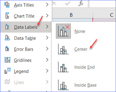
How To Add Data Labels In Excel - sango5460.info To add data labels in excel 2013 or excel 2016, follow these steps: To get there, after adding your data labels, select the data label to format, and then click chart elements > data labels > more options. Using Excel Chart Element Button To Add Axis Labels. After That, Select Insert Scatter (X, Y) Or Bubble Chart > Scatter. Change the format of data labels in a chart To get there, after adding your data labels, select the data label to format, and then click Chart Elements > Data Labels > More Options. To go to the appropriate area, click one of the four icons ( Fill & Line, Effects, Size & Properties ( Layout & Properties in Outlook or Word), or Label Options) shown here.
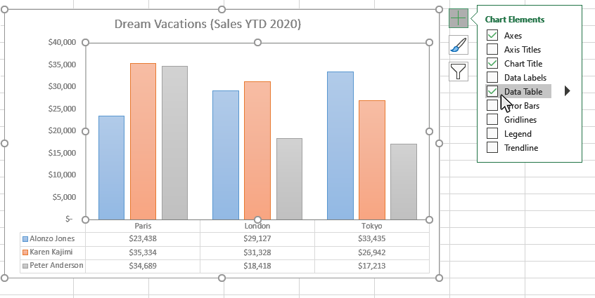
› excel-chart › how-to-add-andHow to Add and Remove Chart Elements in Excel Select the data, go to insert menu --> Charts --> Line Chart. 1: Add Data Label Element to The Chart. To add the data labels to the chart, click on the plus sign and click on the data labels. This will ad the data labels on the top of each point. If you want to show data labels on the left, right, center, below, etc. click on the arrow sign. It ...

How to add data labels on excel
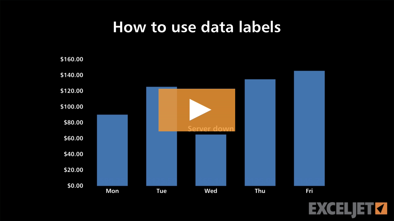
Excel tutorial: How to use data labels When you check the box, you'll see data labels appear in the chart. If you have more than one data series, you can select a series first, then turn on data labels for that series only. You can even select a single bar, and show just one data label. In a bar or column chart, data labels will first appear outside the bar end. › documents › excelHow to hide zero data labels in chart in Excel? - ExtendOffice 1. Right click at one of the data labels, and select Format Data Labels from the context menu. See screenshot: 2. In the Format Data Labels dialog, Click Number in left pane, then select Custom from the Category list box, and type #"" into the Format Code text box, and click Add button to add it to Type list box. See screenshot: 3. How to add text labels on Excel scatter chart axis - Data Cornering Add dummy series to the scatter plot and add data labels. 4. Select recently added labels and press Ctrl + 1 to edit them. Add custom data labels from the column "X axis labels". Use "Values from Cells" like in this other post and remove values related to the actual dummy series. Change the label position below data points.
How to add data labels on excel. How to Print Labels from Excel - Lifewire 05.04.2022 · How to Print Labels From Excel . You can print mailing labels from Excel in a matter of minutes using the mail merge feature in Word. With neat columns and rows, sorting abilities, and data entry features, Excel might be the perfect application for entering and storing information like contact lists.Once you have created a detailed list, you can use it with other … chandoo.org › wp › change-data-labels-in-chartsHow to Change Excel Chart Data Labels to Custom Values? May 05, 2010 · First add data labels to the chart (Layout Ribbon > Data Labels) Define the new data label values in a bunch of cells, like this: Now, click on any data label. This will select “all” data labels. Now click once again. At this point excel will select only one data label. Add a DATA LABEL to ONE POINT on a chart in Excel Click on the chart line to add the data point to. All the data points will be highlighted. Click again on the single point that you want to add a data label to. Right-click and select ' Add data label ' This is the key step! Right-click again on the data point itself (not the label) and select ' Format data label '. How to create Custom Data Labels in Excel Charts - Efficiency 365 Two ways to do it. Click on the Plus sign next to the chart and choose the Data Labels option. We do NOT want the data to be shown. To customize it, click on the arrow next to Data Labels and choose More Options … Unselect the Value option and select the Value from Cells option. Choose the third column (without the heading) as the range.
How to insert or add axis labels in Excel 365 charts (with Example)? Hit the Chart Elements button (marked with a + sign) as shown below. Now, check the box right next to Axis Titles. You'll notice that placeholder for the axis labels, labeled Axis Title will become visible. Double click each of the placeholders and modify the name and font properties as needed. Optionally - modify the chart title as well. Adding Data Labels to Your Chart (Microsoft Excel) - ExcelTips (ribbon) To add data labels in Excel 2013 or later versions, follow these steps: Activate the chart by clicking on it, if necessary. Make sure the Design tab of the ribbon is displayed. (This will appear when the chart is selected.) Click the Add Chart Element drop-down list. Select the Data Labels tool. depictdatastudio.com › how-to-place-labelsHow to Place Labels Directly Through ... - Depict Data Studio Jan 12, 2016 · Click just once on any of those data labels. You’ll see little squares around each data point. Then, right-click on any of those data labels. You’ll see a pop-up menu. Select Format Data Labels. In the Format Data Labels editing window, adjust the Label Position. By default the labels appear to the right of each data point. Excel charts: add title, customize chart axis, legend and data labels Click anywhere within your Excel chart, then click the Chart Elements button and check the Axis Titles box. If you want to display the title only for one axis, either horizontal or vertical, click the arrow next to Axis Titles and clear one of the boxes: Click the axis title box on the chart, and type the text.
How do I add multiple data labels in Excel? - getperfectanswers To add data labels in Excel 2013 or Excel 2016, follow these steps: Activate the chart by clicking on it, if necessary. Make sure the Design tab of the ribbon is displayed. Click the Add Chart Element drop-down list. Select the Data Labels tool. Select the position that best fits where you want your labels to appear. Edit titles or data labels in a chart - support.microsoft.com You can also place data labels in a standard position relative to their data markers. Depending on the chart type, you can choose from a variety of positioning options. On a chart, do one of the following: To reposition all data labels for an entire data series, click a data label once to select the data series. Data Labels in Excel Pivot Chart (Detailed Analysis) Clicking on any Data labels one time will select all of the Data Labels simultaneously. Then right-click on the Data Table and from the context menu, click on the Format Data Labels. Then in the Format Data Labels, go to the Size and Properties. From there, click on the Text Directions. And from the drop-down menu, click on the Rotate all text 270. How can I add data labels from a third column to a scatterplot? Highlight the 3rd column range in the chart. Click the chart, and then click the Chart Layout tab. Under Labels, click Data Labels, and then in the upper part of the list, click the data label type that you want. Under Labels, click Data Labels, and then in the lower part of the list, click where you want the data label to appear.
How to Use Cell Values for Excel Chart Labels
How to Insert Axis Labels In An Excel Chart | Excelchat Figure 4 – How to add excel horizontal axis labels. Now, we can enter the name we want for the primary horizontal axis label; Figure 5 – How to change horizontal axis labels in Excel . How to add vertical axis labels in Excel 2016/2013. We will again click on the chart to turn on the Chart Design tab . We will go to Chart Design and select ...

Add or remove data labels in a chart
How To Create Labels In Excel - allin.northminster.info Creating Labels from a list in Excel YouTube from . 4 quick steps to add two data labels in excel chart. Add a label (form control) click developer, click insert, and then click label. You can now configure the label as required — select the content of. Source: . Select browse in the pane on the right.

How to Add Data Labels in Excel - Excelchat | Excelchat
Custom Chart Data Labels In Excel With Formulas - How To Excel At Excel Follow the steps below to create the custom data labels. Select the chart label you want to change. In the formula-bar hit = (equals), select the cell reference containing your chart label's data. In this case, the first label is in cell E2. Finally, repeat for all your chart laebls.

How to Add Two Data Labels in Excel Chart (with Easy Steps ...
Add data labels to your Excel bubble charts | TechRepublic Right-click the data series and select Add Data Labels. Right-click one of the labels and select Format Data Labels. Select Y Value and Center. Move any labels that overlap. Select the data labels ...

Display Customized Data Labels on Charts & Graphs
Add data labels and callouts to charts in Excel 365 - EasyTweaks.com The steps that I will share in this guide apply to Excel 2021 / 2019 / 2016. Step #1: After generating the chart in Excel, right-click anywhere within the chart and select Add labels . Note that you can also select the very handy option of Adding data Callouts.

How to add or move data labels in Excel chart?
Add a Horizontal Line to an Excel Chart - Peltier Tech 11.09.2018 · This tutorial shows how to add horizontal lines to several common types of Excel chart. We won’t even talk about trying to draw lines using the items on the Shapes menu. Since they are drawn freehand (or free-mouse), they aren’t positioned accurately. Since they are independent of the chart’s data, they may not move when the data changes ...

Add or remove data labels in a chart
How to Print Labels from Excel - Lifewire Choose Start Mail Merge > Labels . Choose the brand in the Label Vendors box and then choose the product number, which is listed on the label package. You can also select New Label if you want to enter custom label dimensions. Click OK when you are ready to proceed. Connect the Worksheet to the Labels

Custom Data Labels with Colors and Symbols in Excel Charts ...
support.microsoft.com › en-us › officeAdd or remove data labels in a chart - support.microsoft.com Depending on what you want to highlight on a chart, you can add labels to one series, all the series (the whole chart), or one data point. Add data labels. You can add data labels to show the data point values from the Excel sheet in the chart. This step applies to Word for Mac only: On the View menu, click Print Layout.

How to add data labels from different column in an Excel chart?
How to add data labels in excel to graph or chart (Step-by-Step) 1. Select a data series or a graph. After picking the series, click the data point you want to label. 2. Click Add Chart Element Chart Elements button > Data Labels in the upper right corner, close to the chart. 3. Click the arrow and select an option to modify the location. 4.

Change the format of data labels in a chart
Add or remove data labels in a chart - support.microsoft.com Depending on what you want to highlight on a chart, you can add labels to one series, all the series (the whole chart), or one data point. Add data labels. You can add data labels to show the data point values from the Excel sheet in the chart. This step applies to Word for Mac only: On the View menu, click Print Layout.

How to Customize Your Excel Pivot Chart Data Labels - dummies
How to Add Data Labels in Excel - Excelchat | Excelchat How to Add Data Labels In Excel 2013 And Later Versions In Excel 2013 and the later versions we need to do the followings; Click anywhere in the chart area to display the Chart Elements button Figure 5. Chart Elements Button Click the Chart Elements button > Select the Data Labels, then click the Arrow to choose the data labels position. Figure 6.
How to Add Data Labels in Excel - Excelchat | Excelchat
› how-to-select-best-excelBest Types of Charts in Excel for Data Analysis, Presentation ... Apr 29, 2022 · Use the moving average trendline if there is a lot of fluctuation in your data. How to add a chart to an Excel spreadsheet? To add a chart to an Excel spreadsheet, follow the steps below: Step-1: Open MS Excel and navigate to the spreadsheet, which contains the data table you want to use for creating a chart. Step-2: Select data for the chart:
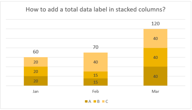
Add Data Labels for Total to Stacked Columns in #Excel | wmfexcel
How to add data labels from different column in an Excel chart? Right click the data series in the chart, and select Add Data Labels > Add Data Labels from the context menu to add data labels. 2. Click any data label to select all data labels, and then click the specified data label to select it only in the chart. 3.

Quick Tip: Excel 2013 offers flexible data labels | TechRepublic
Adding Data Labels To An Excel Chart | MyExcelOnline In our example below, I add a Data Label to a column chart and then I format the data label using CTRL+1. I then select to custom format the numbers so it shows the values as thousands by adding a comma , after each zero and then showing the work k by adding "k" Example Custom Number Format: [$$-1004]#,##0 ,"k" ;- [$$-1004]#,##0 ,"k"

microsoft excel - Adding data label only to the last value ...
› documents › excelHow to add total labels to stacked column chart in Excel? Select and right click the new line chart and choose Add Data Labels > Add Data Labels from the right-clicking menu. See screenshot: And now each label has been added to corresponding data point of the Total data series. And the data labels stay at upper-right corners of each column. 5.

How-to Use Data Labels from a Range in an Excel Chart - Excel ...
How to Add Data Labels to an Excel 2010 Chart - dummies Select where you want the data label to be placed. Data labels added to a chart with a placement of Outside End. On the Chart Tools Layout tab, click Data Labels→More Data Label Options. The Format Data Labels dialog box appears.

Apply Custom Data Labels to Charted Points - Peltier Tech
Format Data Labels in Excel- Instructions - TeachUcomp, Inc. To format data labels in Excel, choose the set of data labels to format. To do this, click the "Format" tab within the "Chart Tools" contextual tab in the Ribbon. Then select the data labels to format from the "Chart Elements" drop-down in the "Current Selection" button group. Then click the "Format Selection" button that ...

How to Add Axis Labels to a Chart in Excel | CustomGuide
how to add data labels into Excel graphs - storytelling with data You can download the corresponding Excel file to follow along with these steps: Right-click on a point and choose Add Data Label. You can choose any point to add a label—I'm strategically choosing the endpoint because that's where a label would best align with my design. Excel defaults to labeling the numeric value, as shown below.

Google Workspace Updates: Get more control over chart data ...
How to Add Two Data Labels in Excel Chart (with Easy Steps) Select the data labels. Then right-click your mouse to bring the menu. Format Data Labels side-bar will appear. You will see many options available there. Check Category Name. Your chart will look like this. Now you can see the category and value in data labels. Read More: How to Format Data Labels in Excel (with Easy Steps) Things to Remember

How to Use Cell Values for Excel Chart Labels
How to add or move data labels in Excel chart? - ExtendOffice In Excel 2013 or 2016. 1. Click the chart to show the Chart Elements button . 2. Then click the Chart Elements, and check Data Labels, then you can click the arrow to choose an option about the data labels in the sub menu. See screenshot:

How to add or move data labels in Excel chart?
How to Use Cell Values for Excel Chart Labels - How-To Geek Select the chart, choose the "Chart Elements" option, click the "Data Labels" arrow, and then "More Options.". Uncheck the "Value" box and check the "Value From Cells" box. Select cells C2:C6 to use for the data label range and then click the "OK" button. The values from these cells are now used for the chart data labels.

How to Add Data Labels to an Excel 2010 Chart - dummies
How to add text labels on Excel scatter chart axis - Data Cornering Add dummy series to the scatter plot and add data labels. 4. Select recently added labels and press Ctrl + 1 to edit them. Add custom data labels from the column "X axis labels". Use "Values from Cells" like in this other post and remove values related to the actual dummy series. Change the label position below data points.

Excel VBA - Add Data Labels from Table body range - Stack ...
› documents › excelHow to hide zero data labels in chart in Excel? - ExtendOffice 1. Right click at one of the data labels, and select Format Data Labels from the context menu. See screenshot: 2. In the Format Data Labels dialog, Click Number in left pane, then select Custom from the Category list box, and type #"" into the Format Code text box, and click Add button to add it to Type list box. See screenshot: 3.

How to Change Excel Chart Data Labels to Custom Values?
Excel tutorial: How to use data labels When you check the box, you'll see data labels appear in the chart. If you have more than one data series, you can select a series first, then turn on data labels for that series only. You can even select a single bar, and show just one data label. In a bar or column chart, data labels will first appear outside the bar end.

How do I add Data Labels for multiple Low Points Only! : r/excel

How to Make Pie Chart with Labels both Inside and Outside ...

Apply Custom Data Labels to Charted Points - Peltier Tech

Creating Pie Chart and Adding/Formatting Data Labels (Excel)

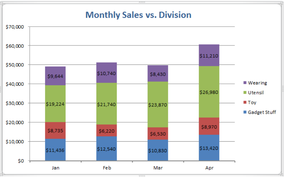
How to Add Total Data Labels to the Excel Stacked Bar Chart ...
Excel tutorial: How to use data labels

Excel Charts: Dynamic Label positioning of line series

Microsoft Excel Tutorials: Add Data Labels to a Pie Chart
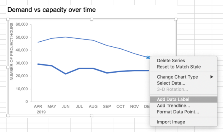
how to add data labels into Excel graphs — storytelling with data

Adding rich data labels to charts in Excel 2013 | Microsoft ...

Using the CONCAT function to create custom data labels for an ...
How to Add Data Tables to a Chart in Excel - Business ...

Adding rich data labels to charts in Excel 2013 | Microsoft ...

Enable or Disable Excel Data Labels at the click of a button ...

Adding rich data labels to charts in Excel 2013 | Microsoft ...

Change the format of data labels in a chart

Excel charts: add title, customize chart axis, legend and ...
How to Add Data Labels to a Chart - ExcelNotes

Chart Data Labels in PowerPoint 2011 for Mac
Post a Comment for "43 how to add data labels on excel"